Chapter 1: Introduction to Time Series Analysis

In this article, we will delve into the fundamentals of time series analysis, emphasizing its relevance in machine learning through practical examples that account for the temporal aspect of data. Forecasting plays a pivotal role in various fields, including finance, weather prediction, and demographic studies, addressing real-world challenges.

Time series models utilize time as a variable, with measurements taken at consistent intervals. The relationship can be expressed as follows:

Z = f(t)

Here, Z represents values Z1, Z2, ... Zn, while "t" denotes time at intervals T1, T2, ... Tn.

Topics to Explore:

• Components of Time Series
• White Noise
• Stationary vs. Non-Stationary Series
• Rolling Statistics and Dickey-Fuller Test
• Differencing and Decomposition
• AR, MA, ARMA, ARIMA Models
• ACF and PACF

The practical applications of time series analysis include tracking daily fuel prices, corporate profits, and quarterly housing market trends.

The Power of Time Series Analysis

Time series analysis is a robust method for making informed forecasting decisions. It assists organizations in anticipating uncertain future events by analyzing data behavior, particularly when combined with data mining techniques.

Chapter 2: Key Components of Time Series

Before diving into modeling time series data, it's essential to understand its core components. Generally, four primary components are identified:

Trends

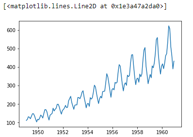
Trends illustrate the upward or downward movement of data values over time. An upward trend indicates increasing values, while a downward trend signifies a decrease.

Example Using Python:

To create a month column with an added day:

data['Month'] = data['Month'].apply(lambda x: dt(int(x[:4]), int(x[5:]), 15))

data = data.set_index('Month')

data.head()

Now, we can visualize the trend using a line chart:

ts = data['#Passengers']

plt.plot(ts)

It’s important to ensure that the index is a date-time data type to make all features dependent on time. For example:

df.month = pd.to_datetime(df.month)

df.set_index('month', inplace=True)

Seasonality and Cycles

Seasonality refers to repetitive patterns in data occurring at regular intervals. For instance, peaks and troughs appearing consistently over time demonstrate seasonality.

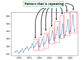
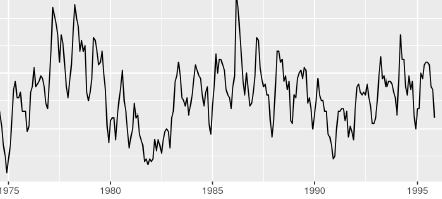
The distinction between seasonality and cycles lies in frequency; seasonality has a fixed periodicity, while cycles do not adhere to a specific timeframe.

Variations and Irregularities

Variations represent non-repeating, short-duration patterns without fixed frequencies.

White Noise

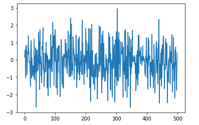
White noise describes segments of a time series where predictions cannot be made due to a lack of correlation between successive values. This segment has a zero mean and constant variance.

For instance, using Python:

import numpy as np

import matplotlib.pyplot as plt

mean_value = 0

std_dev = 1

no_of_samples = 500

time_data = np.random.normal(mean_value, std_dev, size=no_of_samples)

plt.plot(time_data)

plt.show()

Stationary and Non-Stationary Series

A stationary time series maintains a constant mean and variance over time, while a non-stationary series exhibits variability in these parameters.

To convert non-stationary data into stationary form, various methods can be applied.

Rolling Statistics and Dickey-Fuller Test

These tests evaluate the stationarity of a series. Rolling statistics involve examining moving averages and variances, while the Dickey-Fuller test assesses the null hypothesis of non-stationarity.

Example Implementation:

def test_stationarity(timeseries):

rolmean = timeseries.rolling(window=52, center=False).mean()

rolstd = timeseries.rolling(window=52, center=False).std()

plt.plot(timeseries, color='blue', label='Original')

plt.plot(rolmean, color='red', label='Rolling Mean')

plt.plot(rolstd, color='black', label='Rolling Std')

plt.legend(loc='best')

plt.title('Rolling Mean & Standard Deviation')

plt.show(block=False)

dftest = adfuller(timeseries, autolag='AIC')

dfoutput = pd.Series(dftest[0:4], index=['Test Statistic', 'p-value', '#Lags Used', 'Number of Observations Used'])

for key, value in dftest[4].items():

dfoutput['Critical Value (%s)' % key] = value

print(dfoutput)

test_stationarity(data['#Passengers'])

Chapter 3: Advanced Techniques in Time Series Analysis

The first video titled What is Time Series Decomposition? - Time Series Analysis in Python provides a comprehensive overview of decomposition techniques in time series analysis.

The second video, What is Time Series Seasonality | Time Series Analysis in Python, discusses identifying and analyzing seasonal patterns in time series data.

Differencing and Decomposition Techniques

To manage non-stationary data, two primary techniques can be employed: differencing and decomposition. Differencing calculates the change between consecutive observations to stabilize variance.

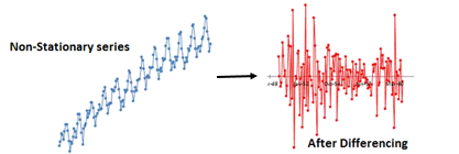
Decomposition involves breaking down a time series into its constituent components through regression analysis.

Time Series Models

Several models exist to fit time series data:

1. AR Model (Auto-Regressive Model): Predicts future values based on past values.
2. MA Model (Moving Average Model): Forecasts based on random error terms.
3. ARMA Model (Auto-Regressive Moving Average): Combines both AR and MA models for better predictions.
4. ARIMA Model (Auto-Regressive Integrated Moving Average): A comprehensive model for analyzing and forecasting time series data.

To illustrate model fitting:

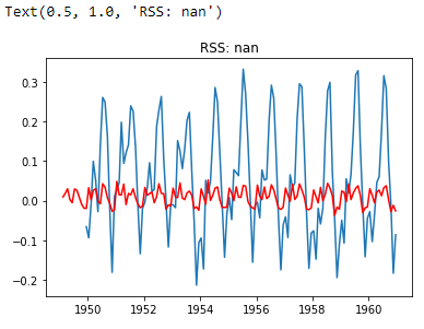
model = ARIMA(ts_log, order=(1, 1, 0))

results_ARIMA = model.fit(disp=-1)

plt.plot(ts_log_mv_diff)

plt.plot(results_ARIMA.fittedvalues, color='red')

plt.title('RSS: %.4f' % sum((results_ARIMA.fittedvalues[1:] - ts_log_mv_diff)**2))

To make predictions using the ARIMA model, follow the steps below:

predictions_ARIMA_diff = pd.Series(results_ARIMA.fittedvalues, copy=True)

predictions_ARIMA_diff_cumsum = predictions_ARIMA_diff.cumsum()

predictions_ARIMA_log = pd.Series(ts_log.ix[0], index=ts_log.index)

predictions_ARIMA_log = predictions_ARIMA_log.add(predictions_ARIMA_diff_cumsum, fill_value=0)

predictions_ARIMA = np.exp(predictions_ARIMA_log)

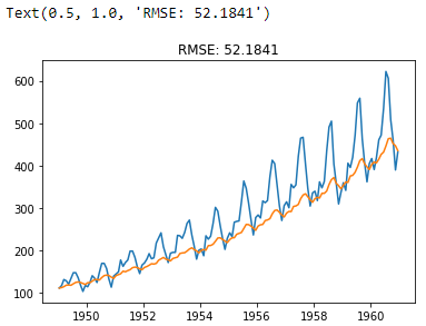
plt.plot(ts)

plt.plot(predictions_ARIMA)

plt.title('RMSE: %.4f' % np.sqrt(sum((predictions_ARIMA - ts)**2) / len(ts)))

Conclusion

In time series modeling, while some models excel in capturing trends, they may struggle with seasonality. This guide serves as an introduction to the essential concepts of time series analysis, supplemented by practical Python examples.

I appreciate your reading. Feel free to connect with me on LinkedIn or Twitter.