A Comprehensive Overview of Box-Counting Techniques
Written on
Box-counting serves as an empirical approach to estimate the fractal dimensions of various objects, images, or sets. The principle is straightforward: we overlay the object with boxes of diminishing sizes and tally how many boxes are needed to cover the object at each scale. This count is termed the “box-counting dimension” or “Minkowski dimension” of the studied object.
For objects with fractal characteristics, there exists a power-law relationship between the box size and the count of occupied boxes. It's crucial to note that while fractal structures suggest an inherent power-law, the presence of a power-law alone does not guarantee fractality.
Before we delve into transforming this size-count relationship into a single dimensional measure, examining concrete examples with familiar objects can enhance our understanding.
Practical Illustrations
The box-counting technique involves progressively covering an image with smaller boxes and tracking the number of occupied boxes at each scale. To clarify the dimension measurement, let’s begin with a simple line.
In Figure 1, we illustrate the process of covering a blue line with boxes of different sizes: lengths of 1, 1/2, 1/4, and 1/8.
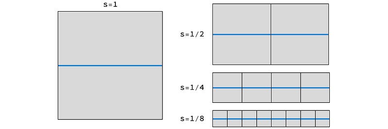
We derive the following counts where N(s) denotes the count for boxes of length s:
N(1) = 1 N(1/2) = 2 = 1/(1/2) N(1/4) = 4 = 1/(1/4) N(1/8) = 8 = 1/(1/8)
This shows that generally, N(s) = 1/s; each time the box's size is halved, the count doubles.
Next, we apply the same method to a filled blue square:
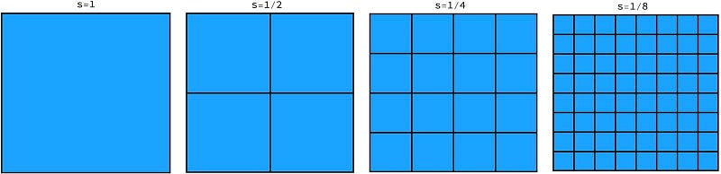
The counts are as follows:
N(1) = 1 N(1/2) = 4 = (1/(1/2))² N(1/4) = 16 = (1/(1/4))² N(1/8) = 64 = (1/(1/8))²
Here, we observe that in general N(s) = (1/s)²; halving the box size increases the count by a factor of 4.
Now, we explore the renowned fractal known as the Sierpinski gasket. This is where things become intriguing.
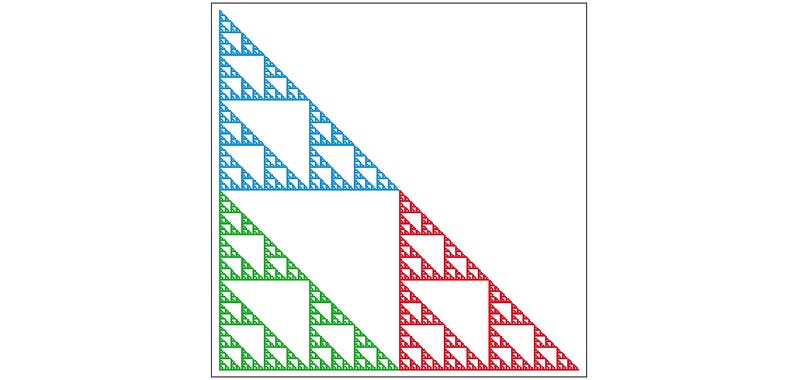
The Sierpinski gasket, also referred to as the Sierpinski triangle or Sierpinski sieve, can be generated in various methods. Named after Polish mathematician Wac?aw Sierpi?ski, it is frequently defined as the limiting shape of an iterated function system (IFS).
In Figure 4, we cover the gasket with the least number of non-overlapping boxes at every scale.
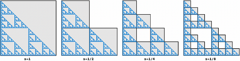
The counts are:
N(1) = 1 N(1/2) = 3 N(1/4) = N((1/2)²) = 9 = 3² N(1/8) = N((1/2)³) = 27 = 3³
Here, the general rule is N((1/2)?) = 3?; halving the box size increases the count by a factor of 3, clearly deviating from the dimensional rules of one or two-dimensional objects.
Understanding Power-Laws
The relationships observed in these examples are indicative of power-laws, where one quantity changes in proportion to a power of another. For counts N, size s, and dimension d, we note:

Taking the logarithm of both sides yields:

Rearranging this gives us:

Equation 1 provides an analytical formula for determining an object's dimension when scaling relationships are established. This is known as the similarity dimension, which can be calculated for self-similar shapes formed from N non-overlapping copies of themselves, each scaled by a contraction factor s.
For the gasket, we find its dimension d = Log(3)/Log(2) ? 1.58496, which intuitively indicates it occupies more space than a line (1-dimensional) yet less than a plane (2-dimensional).
What occurs when we deal with a self-similar object with unknown scaling properties?
Assessing Power-Laws
When scaling properties are unknown, we can verify a power-law by plotting box sizes against their respective counts on a log-log scale. If a power-law is indeed present, the plotted points will align along a straight line indicative of the line of best fit, known as the regression line. The “goodness of fit” is typically quantified using the R-squared value (R²), ranging from 0 to 1 (where 1 indicates a perfect fit). A “good” R² value is context-dependent, varying by field, specific analysis, and data nature.
Assuming the plotted points for size versus count closely align with the regression line, the absolute value of the slope is interpreted as the dimension d of the object being measured. This is due to the transformation of a power-law relation into a linear equation through logarithmic manipulation:

In Equation 2, letting y = Log(N) and x = Log(1/s), we derive the equation of a line, y = mx + b, where d = m and b = 0.
Below are log-log plots of our three examples:
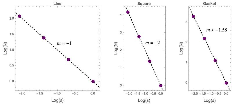
As anticipated, the log-log plots in Figure 5 align with results derived from applying Equation 1.
Coastlines
A classic example of box-counting comes from Benoit Mandelbrot's groundbreaking 1967 paper titled “How Long is the Coast of Britain? Statistical Self-Similarity and Fractional Dimension.”
While conducting his research, Mandelbrot encountered a paper by Lewis Fry Richardson, a multifaceted thinker who pondered the causes of war. He noted that the border length between Spain and Portugal was recorded as 987 km by Spain but 1,214 km by Portugal — a discrepancy of 23%! Such differences are not uncommon.
Richardson discovered that as he reduced the size of his measuring instrument, the length of the border increased. This is logical, as smaller rulers can capture finer features like inlets and coves overlooked by larger rulers, a phenomenon that persists across various scales. This behavior contrasts with familiar Euclidean objects, whose measurements remain consistent regardless of the measuring scale.
Though Mandelbrot did not apply box-counting directly in his paper, his findings were grounded in Richardson's published length measurements from 1961. One of Mandelbrot's key insights was that the observed scaling behavior could be described through the concept of dimension, which offers valuable information regarding the “roughness” of a shape.
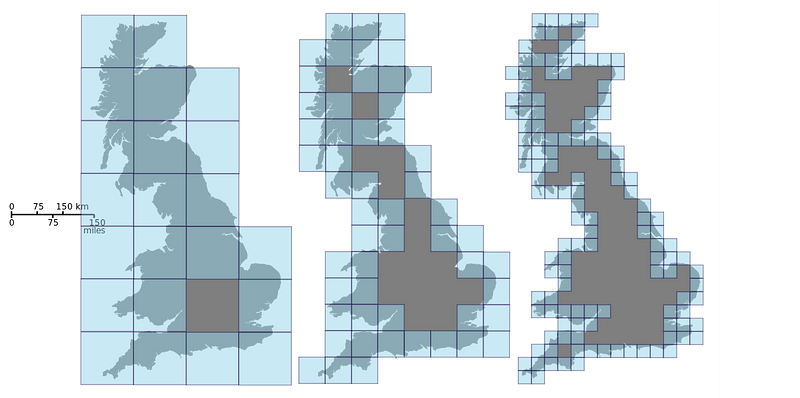
Using Richardson's work, Mandelbrot estimated the dimension of the west coast of Great Britain to be d ? 1.25. Figure 6 depicts the box-counting method applied to Great Britain.
I decided to calculate the box-counting results myself. Figure 7 presents a log-log plot based on map data from Wolfram Research.
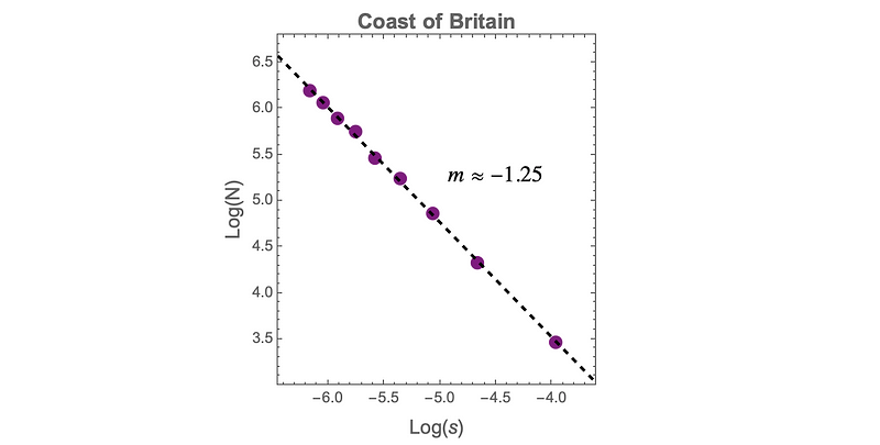
This yields a box-counting dimension of d ? 1.2458, which aligns closely with Mandelbrot's estimate for the west coast. Notably, unlike in Figure 4, where points perfectly matched the regression line, in Figure 7, some points deviate slightly from it. This is expected when measuring natural phenomena, which often exhibit approximate self-similarity rather than strict self-similarity. (Interestingly, this fit is exceptional with R² ? .9991.)
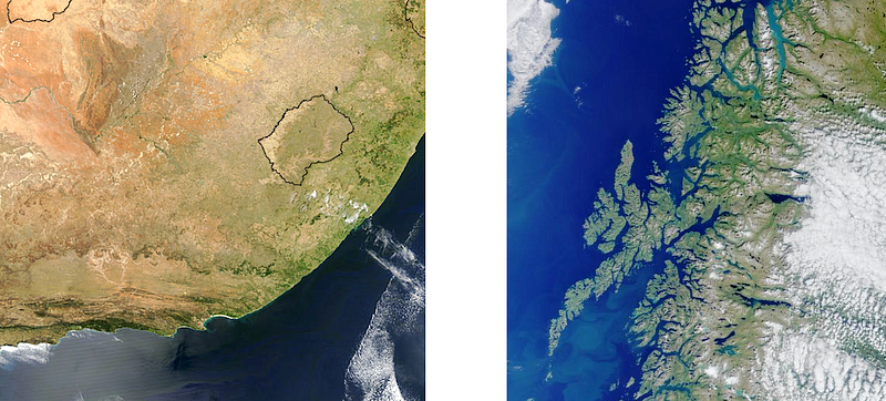
In contrast, South Africa's coastline is relatively smooth, with a dimension of d ? 1.05, while Norway's coastline, characterized by numerous fjords and bays, has a dimension of d ? 1.52.
Broader Applications
Box-counting has numerous variations and can be extended to higher dimensions, finding applications across a wide array of studies.
In nature, this technique aids in exploring river systems, root networks, petri dish colonies, geological formations, biological structures, vegetation patterns, soil arrangements, atmospheric phenomena, and celestial structures.
In industrial contexts, it is utilized in materials science to analyze the microstructure of substances. Understanding structural complexity is essential for grasping their mechanical and physical characteristics. It is also integral to quality control and inspection in manufacturing processes, such as semiconductor fabrication and surface treatment, where assessing roughness, porosity, or irregularities is crucial.
The Koch Curve
To conclude, let's briefly examine a fractal known as the Koch curve, named after Swedish mathematician Niels Fabian Helge von Koch, who studied continuous, non-differentiable curves. This fractal influenced Mandelbrot’s thinking in his 1967 paper.
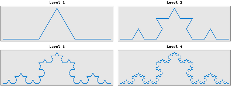
Figure 9 illustrates how the Koch curve is generated. Starting from a straight line, we:
- Remove its middle third, and
- Replace it with a tent shape formed from two segments, each 1/3 the length of the line.
To create the next level of detail, we repeat the “remove middle third”/”replace with tent” operation for each straight segment in the current iteration.
Given that it is composed of four copies, each scaled by 1/3, we can easily compute its similarity dimension (box-counting could also be applied):

The dimension indicates that it is more than a simple line and quantifies its capacity to occupy space. Interestingly, its similarity dimension is close to that of the coastline of Great Britain.
Final Reflections
As a historical note, although Mandelbrot did not employ box-counting in his earlier paper, its impact incited an intellectual surge to explore various natural phenomena where box-counting and its adaptations could be relevant.
Given the widespread use of box-counting in contemporary science and its role in the rigorous analysis of roughness, it's notable that Richardson's pioneering work on coastlines and his insights regarding scale-dependent measurement were largely overlooked by the scientific community at that time.
Fortunately, Mandelbrot's boundless curiosity led him to appreciate the significance of Richardson's groundbreaking contributions. By building on Richardson's foundation, Mandelbrot's explorations laid the groundwork for his influential work in fractal geometry.
- The quote at the beginning of this article is often incorrectly attributed to Albert Einstein.
- Thank you for reading! If you found this article enjoyable, feel free to click the “Applause” icon as many times as you wish. You can also subscribe for my latest content delivered directly to your inbox.